Free Sample Episode

Machine Learning Models for DDoS Detection in Software-Defined Networking: A Comparative Analysis

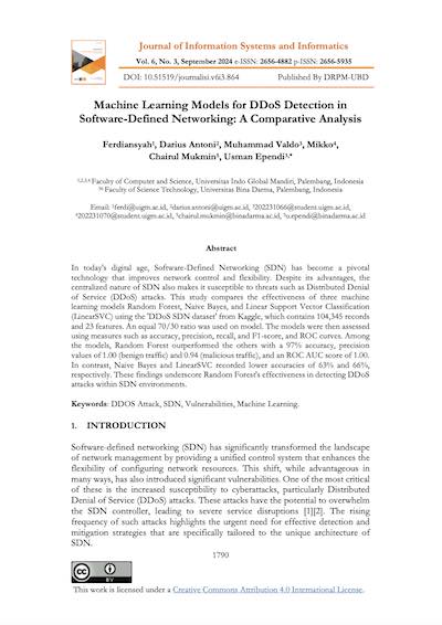
Today's article comes from the Journal of Information Systems and Informatics. The authors are Ferdiansyah et al., from Indo Global Mandiri University, in Indonesia. In this paper, the authors train ML models that can detect DDoS attacks while they're occurring. They train three different versions (using Random Forest, Naive Bayes, and LinearSVC) and benchmark them against each other to see which approach is most effective.

DOI: 10.51519/journalisi.v6i3.864
Book
Book
0:00 0:00
Download this Episode (Right-click, Save-As)

Let’s say you’re in charge of network security at a decent sized eCommerce site. Your company’s big enough that they don’t use AWS or GCP or any other cloud provider, they just run their own machines, maybe in a datacenter or colo-center, or maybe even in a server closet right next to your desk. Either way, that network is a real physical thing that your company relies on, and everyone’s counting on you to protect it.

Everything’s going fine for a while. But then, a week before your biggest sale of the year—a sale that accounts for a huge percentage of your company’s annual profits-–-a week before that, it happens.

You get woken out of bed at 4am. Push notifications. Every service is down. How? Every landing page is offline. Why? Now they’re back up. Now they’re down. You get a frantic call from the SRE on duty. DDoS attack. Small waves at first, rising, then falling, then rising, then nothing. You open your email. There’s a demand, and there’s a threat. That DDoS wave was just a shot across the bow, to get your attention. To show you that they mean business. The attackers, these modern day pirates of the internet seas, give you a matter of days. The bargain is simple. Transfer crypto to them, and do it quickly, or your company’s annual sale will never happen.

What’s your next move? You’ve got time to figure it out. They gave you a few days. But what do you do? Your company’s network interconnects all of the servers and databases that power your site, and exposes itself to the world through your public properties. And it’s entirely your responsibility. Cloudflare can’t save you; you’re not using them. So you think your way through it: That network doesn’t use plain switches or routers, it uses SDN, (software defined networking). So you know you do have an application layer there. A place where could deploy an executable to monitor and block or redirect malicious requests when they come. But how? What logic can you put in place to protect against a DDoS? You can program a solution and deploy it to your network, but what solution?. You know the attack is coming, and you know when it’s coming, but what on earth can you actually do about it?

This paper might hold a clue. The authors’ theory is pretty straightforward: if you can get ahold of sufficiently detailed access logs for the moments that a DDoS attack is happening, then you can use those logs to train a model. A model that can recognize the idiosyncrasies and the feature-shape of individual DDoS requests. Then you can deploy that model right onto your SDN. And when traffic comes in, you can run inference on it, and make determinations in real time as to whether this traffic is likely part of DDoS, which means you can cut the connection and move on, or if it’s normal traffic and should be connected to where it wants to go.

There’s a significant amount of pre-existing literature and research that backs up this idea. But, there’s no clear standard around the best practices for training such a model. Specifically, what algorithm you should use? In this paper the authors make a side-by-side comparison of three different Machine Learning algorithms. Use them all to train separate models, and then test those models to see which algorithm is best for this narrow and particular use-case: running inference inside of an SDN, on incoming traffic data to identify DDoS-related requests in real time.

Before we jump into the nuts and bolts of how they did what they did, we should all get on the same page about what a DDoS attack (a Distributed Denial of Service attack) is and is not. Let’s focus on the DoS part first, the Denial of Service, we’ll come back to the Distributed part in a minute. A Denial of Service attack is named as such because of what it does to the legitimate users of your service. If your servers are receiving a DoS attack and your regular customers are trying to visit your site at the same time, they will likely be denied service. Okay, but how? How can an attacker get you to deny service to your own customers? In a nutshell, they do it by keeping you really busy. There are a few different types of DoS attacks, like UDP floods and HTTP floods, but the one I think is most illustrative (and one of the most common) is called a SYN flood.

Recall that the TCP handshake is a SYN, then a SYN-ACK, then an ACK. In a SYN flood the attacker will send a SYN packet. Your server will receive it, and go “oh hey, someone’s starting the TCP handshake and trying to connect to me” and it will return the SYN-ACK. At this moment, no matter how stateless your userland application is, this handshake occurring in the transport layer has “state” that needs to be kept track of. Who’s connecting, to which port, what SYN they sent, what SYN-ACK you sent etc. It’s a tiny amount of data, but it is there. For most connections it’s a trivial and ephemeral amount of data because after your server sends the SYN-ACK the visitor will respond with the ACK. But most servers are configured to keep that state around and keep the connection open even if the ACK doesn’t come quickly. Most systems assume it’s just a bandwidth issue so they wait to get the ACK back. And while they’re waiting they’re keeping that state somewhere, often in RAM. And in a SYN-flood the attacker won’t follow up with the ACK, it will just turn around, try to connect again separately and then leave your server hanging again. If you repeat this dozens, hundreds, thousands of times, the server starts to take on load. Those open connections do eventually get closed after a timeout period, but they’re not getting closed nearly as quickly as they’re getting opened. So the load grows and grows. And importantly, there is also some limit to the total amount of connections that any one server can keep open at one time. If the attacker can push the open-connections all the way up to that limit, your server will naturally start responding to all future requests (from anyone) with what is effectively a service-denial. We can’t reach this server, we couldn’t connect etc. Those kinds of errors (that your user would see in their browser) are being caused by the fact that you have all these open connections and there’s no room for you to take on any future connections. But as far as your site visitors are concerned, all they know is you denied them service. This attack is bad enough on its own, but can easily be shutdown if the attack is just coming from one other machine. This is where the “Distributed” part comes in. If an attacker can control a distributed botnet (often consisting of infected computers owned by innocent bystanders), then they can run this attack on you from a multitude of IPs and locations all at once, completely overwhelming your ability to do anything about it.

The solution that these authors are advocating that you build, would be installed upstream of your application servers. It’d be installed on the actual networking infrastructure (switches, routers etc). Since modern versions of those systems leverage SDN, you can deploy a model to your networking layer without touching your userland applications.

So how did they train this model? They started by pulling down a dataset from Kaggle, the DDOS SDN Dataset. This was perfect for a few reasons: namely it was the type of access data that an SDN-based application would actually have access to in real time, and the data was labeled. There were about a hundred thousand rows, ~60% were requests that were part of a DDoS, and ~40% were just normal users. And in addition to that column there were 22 other columns of categorical and numerical data. Everything from source IP address, to packet-count, to packet-rate, to total kbps. Basically all of the metadata about the request. These 22 columns of meta-data became the features that they’d use in model training.

The CSV data was nearly ready to be imported into their training bench as-is, they just needed to convert the categorical data into numerical values and split the dataset into 70% training, 30% testing and validation. Importantly, they didn’t do any feature selection. They didn’t narrow down this group of 22 columns at all, they just used them all. We’ll come back to the effects that might have had later.

Anyway, after the preprocessing they were able to actually train. The training process is something they ran through three times: once for each of the training algorithms they wanted to benchmark. Namely: Random Forest, Naive Bayes, and LinearSVC. If that doesn’t sound familiar, that's a dedicated linear classifier derived from SVM (the support vector machine). Each of these training algorithms take a different approach. As training data is fed in, they’ll all make slightly different decisions about how the shape of that new data should (or shouldn’t) tune the weights of the model. Some algorithms are aggressive. Some are conservative. Some create big models, some create small. Some look at the relationships between features, others consider each feature to be independent of each other. So what the authors end up with is three models that can all be deployed for the same use-case, but will infer different outputs for any given set of inputs. Since they looked at and considered their training data differently, the inference they run looks at new test data differently, generating different results.

To compare the models to each other, the authors used 4 metrics and 2 visualizations. Here are the metrics:

  1. Accuracy: The number of correct predictions (both true positives and true negatives) out of the total predictions.
  2. Precision: The number of correct positive predictions out of all positive predictions made.
  3. Recall: The number of correct positive predictions out of all actual positive instances.
  4. F1 Score: The harmonic mean of precision and recall, providing a balance between the two.

And for the visualizations they generated an RoC curve, and a confusion matrix. An RoC curve is a graphical plot that shows the trade-off between the true positive rate (recall) and the false positive rate at various threshold settings. It helps to assess the model's performance across different classification thresholds. A confusion matrix is a table that shows the number of true positives, true negatives, false positives, and false negatives, providing a detailed breakdown of the model's classification performance.

Compared side by side, the results stared them in the face. You can find the raw result data in Table 2 in the PDF, but let me summarize it very briefly:

  • Naive Bayes: All metrics between 0.35 and .081. Most importantly, accuracy was 0.63.
  • LinearSVC: All metrics between 0.55 and .083. Accuracy was 0.66.
  • Random Forest: All metrics between 0.95 and 1.0. Accuracy was 0.97.

So clearly the winner was Random Forest. Right? Well, yes and no.

The key piece of missing information here is that these three models, since they're different sizes and different levels of complexity, don't run inference at the same speeds. Naive Bayes is the least accurate, sure, but it’s also the fastest. Random Forest is by far the most accurate, but it’s slow and resource hungry. And remember this application would be living in an SDN environment, likely highly resource constrained. LinearSVC is somewhere between those two in terms of accuracy and also in terms of speed.

So is there a clear winner? I’d say no, for three reasons:

  1. As I just alluded to, “winner” depends on what your deployed environment can accommodate. The most accurate model in the world isn’t worth anything if it’s too slow on the available hardware to be usable.
  2. The assumption that the implementation of these models would be mutually exclusive of each other is false. You can use two of them, or all of them, and it might be a significantly better solution than using just one. Bayes can be the first line of defense since it’s so fast, but then the data can be thrown over to the larger models for more thorough checking asynchronously. Bayes will provide at least some level of front-line protection and will be able to potentially mitigate against attacks while your larger models are validating the traffic more thoroughly.
  3. While you could do a layered approach, you could also do a swap-out at key times. Even Cloudflare has an “I’m under attack” button that you can click in your dashboard to tell them that your site is experiencing such an event. And that allows them to use a different level of security procedures and analysis on the traffic than they would when times are fine. In our case you could activate different models depending on the threat level and the overall likelihood of an attack at that moment.

To bring it back to the ransom attack you hypothetically experienced at the beginning of this talk. These authors would say that the shot-across-the-bow was actually your lucky day. Because in sending you that DDoS sample, you got enough data to stop the big one in its tracks. When you got the 4am demand-letter, you could simply say: “You know what? I’m going to train a model based on the sample attack they just carried out, then deploy that model to our SDN. Maybe I’ll even do several of them. In the morning. But right now, I can go back to bed.”